(Intro) Stop guessing. Start calculating.
How to Calculate Velocity Banking Savings in Excel (Step-by-Step DIY Guide)

If you are reading this, you probably know that Velocity Banking is the most powerful strategy to pay off a 30-year mortgage in 5-7 years. But there is a catch: The math is unforgiving.
One wrong decimal point in your amortization schedule could cost you thousands in miscalculated interest savings.
In this technical guide, I will walk you through how to build your own velocity banking calculator in Excel from scratch. I will share the exact formulas I used during my 15 years in institutional banking.
⚠️ Quick Note: Don’t want to spend 4 hours building complex formulas? [Check out our automated Mortgage Killer Kit™ here] (Link para a Home/Produto). It includes the pre-built Excel Tracker and PDF Guide, ready to use immediately.
(H2) The Math: Amortized vs. Simple Interest
Before opening Excel, you must understand the two opposing forces at play:
- Your Mortgage (Amortized Interest): This is front-loaded. In the first 5-7 years, the majority of your payment goes to interest, not principal.
- Your HELOC (Simple Interest): Calculated daily based on the average balance.
The goal of your spreadsheet is to determine the exact moment (the “crossover point”) when using a HELOC chunk saves more money than it costs.
(H2) Step-by-Step: Building the Spreadsheet
Open a blank Excel or Google Sheets file. We are going to build a dynamic tracker.
Step 1: Set Up Your Input Variables In cells A1 through B5, create fields for your static numbers. You will reference these later.
- Mortgage Balance: (e.g., $200,000)
- Mortgage Rate: (e.g., 6.5%)
- HELOC Rate: (e.g., 8.5%)
- Monthly Income: (Net)
- Monthly Expenses: (Everything except the mortgage)
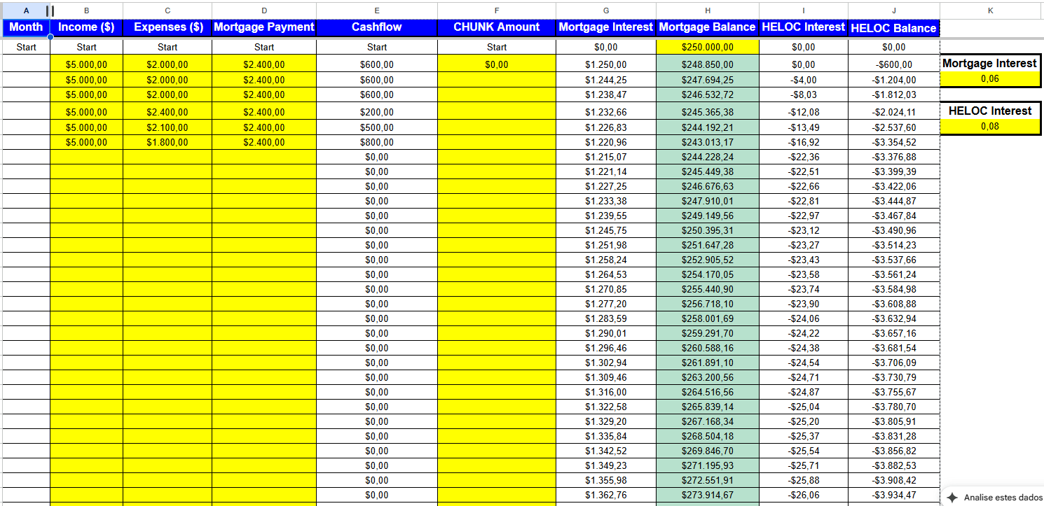
Step 2: Create the Columns In Row 10, create these headers. This is the engine of your calculator:
- Column A: Month (1, 2, 3…)
- Column B: Cash Flow (Income – Expenses)
- Column C: Chunk Amount (The transfer from HELOC to Mortgage)
- Column D: Mortgage Interest (The cost of the loan)
- Column E: Mortgage Balance (The dying debt)
- Column F: HELOC Interest (The cost of the line)
- Column G: HELOC Balance (The revolving debt)
(H2) The Velocity Banking Formulas
Here is where it gets technical. You need to program the logic of the “Chunk.”
1. Calculating Mortgage Interest (Column D): You cannot just divide by 12. You must calculate based on the remaining balance after the chunk is applied. =PreviousBalance * (MortgageRate / 12)
2. The HELOC Logic (Column G): This is the hardest part. Your HELOC balance fluctuates daily as you deposit your paycheck and pay bills. In a simple monthly view, use this formula logic: =PreviousHELOC + NewChunk + HELOCInterest - FreeCashFlow
(Note: If this formula returns a negative number, it means your HELOC is paid off and ready for the next chunk).
(H2) Watch: The Spreadsheet in Action
If you are visual, watch this breakdown of how the columns interact when you apply a $10,000 chunk against a $200,000 mortgage.
(H2) The Risk of DIY Spreadsheets (Why Most Fail)
I have audited hundreds of client spreadsheets. The 3 most common errors I see in “DIY” velocity banking calculators are:
- The “Float” Error: Forgetting that HELOC interest is calculated on the Average Daily Balance, not the month-end balance. This often makes your DIY sheet look more optimistic than reality.
- Broken Links: One drag-and-drop error in Row 36 can mess up your projection for Year 7.
- Tax & Escrow: Most DIY sheets forget that property taxes increase over time, which eats into your cash flow.
Is it worth the risk? Velocity Banking works, but only if the numbers are precise. You are dealing with your largest asset—your home. This is not the place for “guesstimates.”
(H2) Save Time & Get Precision: The Mortgage Killer Kit™
Instead of building this from scratch and worrying about broken formulas, you can download my professional-grade tool.
I have spent 500+ hours coding and refining the Mortgage Killer Tracker. It handles:
- ✅ Variable HELOC rates.
- ✅ Automatic “Chunk” suggestions.
- ✅ Visual dashboards (Debt-Free Date).
- ✅ 100% Error-free amortization logic.
It costs $27 (less than a takeout dinner).
[Download the Mortgage Killer Kit & Calculator Here] (Link para o Produto/Checkout)
❓ Frequently Asked Questions
Can I do this in Google Sheets?
Yes, the logic is the same. However, Google Sheets can sometimes be slower with iterative calculations used in advanced amortization modeling.
How do I calculate the Chunk size?
A general rule of thumb is to keep your Chunk size roughly equal to 3-4 months of your net income, provided your HELOC limit allows it.
Need more help?
Read our [Velocity Banking for Beginners Guide] to understand the strategy before you build the math.

About the Author Michael
MBA in Quantitative Finance – Wharton School (University of Pennsylvania)."I built products for the banks. Now, I dismantle them for you."Michael Schmidt is a veteran financial strategist and the architect of the Mortgage Killer Method.With over 15 years of experience inside America's largest lending institutions, Michael worked behind closed doors structuring mortgage backed-securities. He saw firsthand how the "30-year fixed" system is engineered to prioritize institutional profit over homeowner equity.In 2015, Michael walked away from Wall Street with a clear objective: to reverse-engineer banking mathematics for the average American family. He specializes in aggressive principal reduction strategies, using HELOCs to cut amortization timelines by decades.Michael brings German precision to debt management. His frameworks are not theories—they are mathematical certainties. To date, he has helped over 1,500 families reclaim an estimated $50 million in interest from the banking system.Expertise: Strategic Debt Elimination, Amortization Mechanics, Cash Flow Optimization.Background: Former VP of Lending Strategies.